
2.5 Heisenberg’s Uncertainty Principle and Quantum Numbers
🧠 Lesson 5: Heisenberg’s Uncertainty Principle and Quantum Numbers
Chapter: Atomic Structure
Student Learning Outcomes (SLOs 2.5.1 – 2.5.4)
Learning Objectives
- Describe the concept of an orbital based on Heisenberg’s uncertainty principle.
- Compare the terms “orbit” and “orbital.”
- Describe the four quantum numbers: principal, azimuthal, magnetic, and spin.
- Use quantum numbers to deduce electron position and distribution.
📺 Video Lesson: Quantum Numbers and Electron Orbitals
This video explains the orbital model, Heisenberg’s uncertainty principle, and the four quantum numbers, showing how electrons are distributed in atoms.
1. Heisenberg’s Uncertainty Principle (SLO 2.5.1)
In 1927, Werner Heisenberg proposed a principle that fundamentally dismantled the classical view of atomic physics. The Heisenberg uncertainty principle states that it is physically impossible to simultaneously measure both the exact position ($x$) and the exact momentum ($p$) of a microscopic particle like an electron. Mathematically, this relationship is expressed as:
$$\Delta x \cdot \Delta p \ge \frac{h}{4\pi}$$
Where $\Delta x$ is the uncertainty in position, $\Delta p$ is the uncertainty in momentum, and $h$ is Planck’s constant. Because the product of these uncertainties must be greater than or equal to a constant value, improving the precision of one measurement inherently destroys the precision of the other.
Because we cannot know exactly where an electron is and where it is going at the same time, we cannot visualize electrons traveling in fixed, planetary paths. Instead, quantum mechanics treats electrons as a “cloud” of negative charge, defining specific regions of space called orbitals where the probability of finding an electron is exceptionally high (usually above 90%).
⚡ Quick-Fact: A Fundamental Limit, Not a Flaw
The uncertainty principle is not a limitation of our laboratory instruments or human error. It is a fundamental property of the wave-particle duality of nature. To “see” an electron, you must bounce a photon of light off it. The energy of that photon is so massive relative to the electron that the collision instantly changes the electron’s momentum!
2. Orbit vs Orbital (SLO 2.5.2)
The transition from the Bohr model to the Quantum Mechanical model requires a strict differentiation between two easily confused terms: the Orbit and the Orbital.
| Feature | Orbit (Classical / Bohr Model) | Orbital (Quantum Model) |
|---|---|---|
| Definition | A well-defined, 2D circular path around the nucleus. | A 3D region of space with a high probability of finding an electron. |
| Uncertainty Principle | Violates Heisenberg’s Principle (assumes exact position and momentum). | Strictly obeys Heisenberg’s Principle (relies purely on probability). |
| Shape | Always circular or elliptical. | Complex 3D geometries (spherical, dumbbell, cloverleaf). |
| Capacity | Can hold $2n^2$ electrons. | Can hold a maximum of exactly 2 electrons (with opposite spins). |
3. Quantum Numbers (SLOs 2.5.3 & 2.5.4)
To perfectly describe the energy, position, and behavior of any electron within an atom, physicists use a mathematical “address” consisting of four specific Quantum Numbers. No two electrons in an atom can have the exact same set of four quantum numbers (Pauli Exclusion Principle).
3.1 Principal Quantum Number ($n$)
This determines the primary energy level or shell of the electron. It dictates the overall distance of the electron from the nucleus. Allowed values are integers: $n = 1, 2, 3, \dots$ As $n$ increases, the orbital becomes larger, and the electron’s energy increases. The maximum number of electrons an energy level can hold is given by $2n^2$.
3.2 Azimuthal / Angular Momentum Quantum Number ($\ell$)
This determines the 3D shape of the subshell where the electron resides. The allowed values of $\ell$ depend on $n$ and range from $0$ to $(n-1)$. Each numerical value corresponds to a specific letter designation:
- $\ell = 0 \rightarrow$ s subshell (spherical shape)
- $\ell = 1 \rightarrow$ p subshell (dumbbell shape)
- $\ell = 2 \rightarrow$ d subshell (double-dumbbell/clover shape)
- $\ell = 3 \rightarrow$ f subshell (complex multi-lobed shape)
3.3 Magnetic Quantum Number ($m_\ell$)
This specifies the spatial orientation of a specific orbital within a magnetic field. The allowed values depend on $\ell$ and range from $-\ell$ through $0$ to $+\ell$. For example, if an electron is in a $p$ subshell ($\ell = 1$), the possible $m_\ell$ values are $-1, 0, +1$. This tells us there are exactly three distinct $p$ orbitals ($p_x, p_y, p_z$) oriented along different spatial axes.
3.4 Spin Quantum Number ($m_s$)
Unlike the first three, this number describes an intrinsic property of the electron itself, not its orbital. Electrons generate a tiny magnetic field, acting like miniature magnets. They can only possess one of two spin states: $+\frac{1}{2}$ (“spin-up”) or $-\frac{1}{2}$ (“spin-down”). If two electrons share the exact same orbital, they must have opposite spins to minimize magnetic repulsion.
📊 Concept Diagram: Quantum Numbers and Orbital Shapes
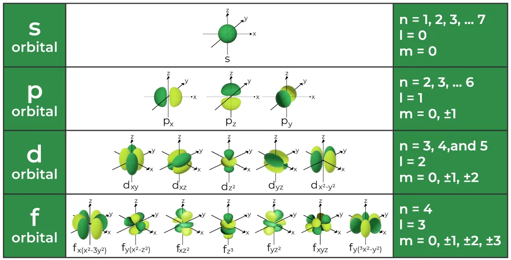
Different orbital shapes and spatial orientations corresponding to specific azimuthal ($\ell$) and magnetic ($m_\ell$) quantum numbers.
🎯 AKU Exam Insights
- Identifying Impossible States: A very common multiple-choice question format asks you to identify the “impossible” set of quantum numbers. Always check the $\ell$ value first. The value of $\ell$ can NEVER be equal to or greater than $n$. (e.g., If $n=2$, $\ell$ cannot be $2$).
- Orbital Capacity vs. Shell Capacity: Read questions carefully! The maximum number of electrons in a shell is $2n^2$. However, the maximum number of electrons in any single orbital (regardless of whether it is an $s, p, d,$ or $f$ orbital) is always exactly 2.
4. Concept Check
1. According to Heisenberg’s Uncertainty Principle, what happens when the measurement of an electron’s position becomes incredibly precise?
Check Answer & Explanation
Explanation: Because the product of $\Delta x$ and $\Delta p$ must be greater than or equal to a constant ($\frac{h}{4\pi}$), an extremely small $\Delta x$ (high precision in position) forces $\Delta p$ (uncertainty in momentum) to become extremely large to maintain the inequality.
2. Which of the following is a defining characteristic of an “orbital” compared to a Bohr “orbit”?
Check Answer & Explanation
Explanation: The quantum mechanical model abandons fixed pathways (orbits) and embraces probability density. An orbital is simply a mathematical boundary containing the space where an electron will be found roughly 90% of the time.
3. Which of the following sets of quantum numbers $(n, \ell, m_\ell, m_s)$ is theoretically IMPOSSIBLE for an electron?
Check Answer & Explanation
Explanation: The magnetic quantum number ($m_\ell$) is strictly constrained by the azimuthal quantum number ($\ell$), where $m_\ell$ can only be values from $-\ell$ to $+\ell$. If $\ell = 0$ (an $s$ orbital), then $m_\ell$ MUST be $0$. It cannot be $+1$.
📌 Lesson Summary
- Heisenberg’s Uncertainty Principle fundamentally limits our simultaneous knowledge of an electron’s precise position and momentum, proving that electrons do not travel in fixed orbits.
- An orbit is a classical, 2D circular path, while an orbital is a 3D region of high probability dictated by quantum mechanics.
- The Principal quantum number ($n$) defines the main energy shell and size.
- The Azimuthal quantum number ($\ell$) dictates the 3D geometry and shape of the subshell ($s, p, d, f$).
- The Magnetic quantum number ($m_\ell$) defines the specific spatial orientation of the orbital along the $x, y,$ or $z$ axes.
- The Spin quantum number ($m_s$) describes the intrinsic magnetic spin of the electron itself ($+\frac{1}{2}$ or $-\frac{1}{2}$).
➡ Coming Next
Lesson 6 — Dual Nature of Electron
🚀