
Physical Quantities and Measurement
Learning Objectives
After studying this chapter you should be able to:
- Distinguish between base and derived physical quantities
- Use the International System of Units (SI) and perform unit conversions
- Apply scientific notation and understand order of magnitude
- Perform dimensional analysis to check equations and derive relationships
- Differentiate between scalars and vectors
- Perform vector operations including addition, subtraction, and resolution into components
- Calculate scalar (dot) and vector (cross) products
- Understand and apply conditions for equilibrium
- Calculate torque as a vector product
1. Physical Quantities and Measurement
Physics is the foundation of all natural sciences. It provides the language and tools needed to describe nature quantitatively, from the motion of planets to the behavior of subatomic particles. This chapter introduces the core ideas that will be used throughout mechanics, thermodynamics, electricity, and modern physics.
In the syllabus, this topic includes: physical quantities and measurement; base and derived quantities; SI and technical units; prefixes; scientific notation and unit conversions; scalars and vectors with vector operations. Mastery of these ideas is essential, as every physical law is expressed through measured quantities.
Why Physics Matters
Physics helps us understand how the world works. It’s used in many important areas:
- Space Technology: Sending rockets to the Moon, calculating escape velocity, and keeping satellites in orbit using gravitational and centripetal force principles.
- Nanotechnology: Manipulating matter at atomic and molecular scales for applications such as semiconductors and targeted drug delivery.
- Medical Physics: Using X-rays, MRI, CT scans, ultrasound, and radiation therapy, all of which rely on precise physical measurements.
1.1 Base and Derived Quantities
A physical quantity is any property of a system that can be measured and expressed numerically together with a unit. Measurement always involves comparing an unknown quantity with a standard quantity of the same kind.
Examples of physical quantities include length, mass, time, force, energy, temperature, and electric current.
Physical quantities are divided into two main categories:
base (fundamental) quantities, which are defined independently, and derived quantities, which are obtained by combining base quantities through mathematical relationships.
SI Base Units
The International System of Units (SI) is the globally accepted system of measurement used in science,
engineering, and medicine. It ensures uniformity and consistency of measurements across the world.
SI is based on seven base quantities, each with a defined unit.
| Quantity | Unit | Symbol |
|---|---|---|
| Length | meter | m |
| Mass | kilogram | kg |
| Time | second | s |
| Electric Current | ampere | A |
| Temperature | kelvin | K |
| Amount of substance | mole | mol |
| Luminous intensity | candela | cd |
Derived Units
Derived quantities are defined in terms of base quantities. Their units are obtained by algebraic
combinations of SI base units.
- Velocity: m/s — rate of change of displacement with time.
- Acceleration: m/s² — rate of change of velocity with time.
- Force: N = kg·m/s² — interaction that causes a change in motion.
- Energy: J = kg·m²/s² — capacity to do work.
- Pressure: Pa = N/m² — force per unit area.
1.2 SI Units, Prefixes, Scientific Notation, and Conversions
The SI system also includes derived units with special names (such as newton, joule, and pascal)
and a standardized set of prefixes to represent powers of ten. This allows physicists to express extremely large quantities (such as astronomical distances) and extremely small quantities (such as atomic dimensions) conveniently.
Scientific notation expresses numbers as a product of a number between 1 and 10 and an integer power of 10.
It reduces errors and makes calculations simpler, especially in physics problem-solving.
| Prefix | Symbol | Factor | Scientific Notation |
|---|---|---|---|
| mega | M | 1,000,000 | 10⁶ |
| kilo | k | 1,000 | 10³ |
| milli | m | 0.001 | 10⁻³ |
| micro | μ | 0.000001 | 10⁻⁶ |
Unit conversion is performed by multiplying by appropriate conversion factors so that the numerical value
changes while the physical quantity remains the same. Dimensional consistency must always be maintained.
Unit conversions and dimensional analysis are the “common sense” of science and math. They ensure that when you calculate something, the numbers actually mean what you think they mean.
Unit Conversions: The “Identity” Trick
A unit conversion changes the label of a measurement (like inches to centimeters) without changing the actual amount. This works because of a mathematical trick: multiplying by 1.
In unit conversion, we use Conversion Factors. A conversion factor is a fraction where the top and bottom are equal amounts, so the fraction itself equals $1$.
-
Example: Since $1 \text{ foot} = 12 \text{ inches}$, the fraction $\frac{1 \text{ ft}}{12 \text{ in}}$ is essentially $1$.
The Rule of Cancellation
To convert units, you set up your fraction so the unit you don’t want is on the opposite side (top vs. bottom) so they “cancel out.”
Example: Convert $36$ inches to feet.
$$36 \text{ in} \times \frac{1 \text{ ft}}{12 \text{ in}} = \frac{36}{12} \text{ ft} = 3 \text{ ft}$$
The “inches” on top and bottom cancel out, leaving only “feet.”
1.3 Scalars and Vectors
Physical quantities can also be classified as scalars and vectors.
Scalars are completely described by magnitude alone, whereas vectors require both magnitude and direction.
Examples and Vector Operations
- Scalars: mass, time, temperature, energy, speed.
- Vectors: displacement, velocity, acceleration, force, momentum.
Vector operations include vector addition and subtraction, as well as resolving vectors into components
along perpendicular axes. These operations are fundamental in mechanics.
(Diagram: vector addition, parallelogram method, and resolution of vectors)
1.4 Measurement Errors and Uncertainty
Types of Errors
- Systematic Errors: consistent deviations caused by faulty instruments or incorrect calibration.
- Random Errors: unpredictable variations arising from limitations of measurement techniques.
Precision vs Accuracy
Precision refers to the closeness of repeated measurements to each other, while accuracy indicates how close a measurement is to the true or accepted value.

1.5 Dimensional Analysis
Dimensional analysis is a powerful method used to verify equations, derive relationships between physical quantities,
and convert units by ensuring dimensional consistency.
| Quantity | Dimensions |
|---|---|
| Velocity | [L][T]⁻¹ |
| Acceleration | [L][T]⁻² |
| Force | [M][L][T]⁻² |
| Energy | [M][L]²[T]⁻² |
| Power | [M][L]²[T]⁻³ |
Dimensional Analysis: The Big Picture
While unit conversion is about changing labels, Dimensional Analysis is a problem-solving method that uses those units to navigate through complex calculations. It treats units like algebraic variables.
The Core Dimensions
In physics, almost everything can be broken down into three fundamental dimensions:
-
Mass [M]: grams, kilograms, pounds.
-
Length [L]: meters, miles, inches.
-
Time [T]: seconds, hours, days.
Why it Matters (The Sanity Check)
You can use dimensional analysis to check if an equation is even possible. This is called the Principle of Homogeneity. It states that you can only add or subtract quantities if they have the same dimensions. You can’t add $5$ kilograms to $10$ meters—it’s “apples and oranges.”
Example: Checking a formula
Is the formula $\text{Distance} = \text{Speed} \times \text{Time}$ correct?
-
Dimensions of Distance: $[L]$
-
Dimensions of Speed: $\frac{[L]}{[T]}$ (Length per Time)
-
Dimensions of Time: $[T]$
- The Math: $\frac{[L]}{[T]} \times [T] = [L]$Since both sides equal $[L]$, the formula is dimensionally consistent!
3. How to Solve Any Problem Step-by-Step
If you are faced with a complex word problem, follow this “Grid” method:
-
Identify the Given: What number and unit are you starting with?
-
Identify the Goal: What unit do you want at the end?
-
Find Conversion Factors: What links the starting unit to the goal?
-
Set up the “Train Tracks”: Line them up so units cancel diagonally.
-
Calculate: Multiply everything on the top, then divide by everything on the bottom.
| Starting Value | Factor 1 | Factor 2 | Final Result |
| $2 \text{ days}$ | $\frac{24 \text{ hours}}{1 \text{ day}}$ | $\frac{60 \text{ minutes}}{1 \text{ hour}}$ | $2,880 \text{ minutes}$ |
2. Scalars and Vectors
In physics, quantities are not all described in the same way. Some quantities only require a numerical value,
while others also need a direction to be fully specified. This distinction is crucial in mechanics, electricity,
and fields, and IMAT frequently tests the ability to identify, manipulate, and interpret these quantities correctly.
Scalars and vectors form the mathematical language of physics. Understanding their properties and operations
is essential before studying motion, forces, momentum, and energy.
Scalars vs. Vectors
A scalar quantity is completely described by its magnitude (numerical value and unit).
A vector quantity, on the other hand, requires both magnitude and direction.
Confusing these two is a common IMAT trap, especially in kinematics and dynamics.
| Scalars | Vectors |
|---|---|
|
|
Key IMAT insight: Speed is a scalar, but velocity is a vector. Distance is scalar, displacement is vector.
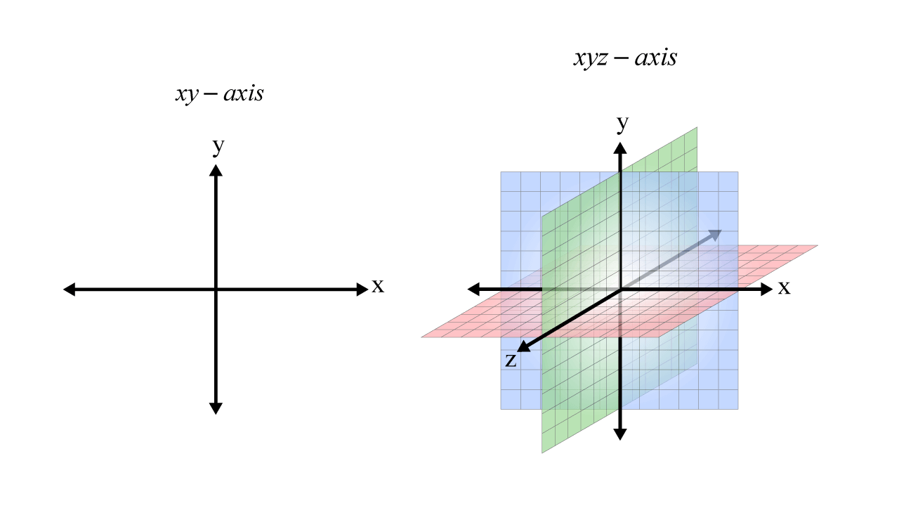
2.1 Cartesian Coordinate System
To describe vectors quantitatively, a reference system is required. The Cartesian coordinate system
allows vectors to be represented using numerical components along mutually perpendicular axes.
Two-Dimensional System (2D)
- Defined by two perpendicular axes: x-axis (horizontal) and y-axis (vertical)
- Their intersection defines the origin O(0,0)
- A point P is located by coordinates (x, y)
- A vector is described by its magnitude and the angle θ with the positive x-axis

Three-Dimensional System (3D)
- Adds a third axis (z-axis) perpendicular to both x and y
- Used to describe motion and forces in space
- A point P is located by coordinates (x, y, z)
- Vector direction may be specified by angles with each axis
2.2 Vector Types and Operations
Types of Vectors
- Resultant Vector: A single vector that has the same effect as multiple vectors acting together
- Negative Vector: Same magnitude but opposite direction to a given vector
- Unit Vector: Magnitude equal to 1; used to represent direction only (î, ĵ, k̂)
- Null Vector: Zero magnitude; direction is undefined
- Position Vector: Vector drawn from the origin to a point in space
- Equal Vectors: Same magnitude and same direction, regardless of position
Head-to-Tail Vector Addition
- Place the tail of the second vector at the head of the first
- The resultant vector goes from the tail of the first to the head of the last
- Vector addition is commutative: $$\vec{A} + \vec{B} = \vec{B} + \vec{A}$$

Resolution into Rectangular Components
Any vector can be expressed as the sum of perpendicular components along the coordinate axes.
This method simplifies vector addition and subtraction.
$$A_y = A\sin\theta$$
where A is the magnitude of the vector and θ is the angle measured from the positive x-axis.
2.3 Scalar Product (Dot Product)
The scalar (dot) product of two vectors results in a scalar quantity.
It measures how much one vector acts in the direction of another.
Definition:
$$\vec{A} \cdot \vec{B} = AB\cos\theta$$
where θ is the angle between the two vectors.
Special Cases
- θ = 0° (parallel): maximum positive value
- θ = 90° (perpendicular): dot product equals zero
- θ = 180° (opposite directions): maximum negative value
Component Form
2.4 Vector Product (Cross Product)
The vector (cross) product of two vectors results in a vector that is perpendicular
to the plane containing the original vectors. It is fundamental in rotational mechanics and electromagnetism.
Definition:
$$\vec{A} \times \vec{B} = AB\sin\theta\,\hat{n}$$
where $\hat{n}$ is a unit vector perpendicular to both A and B, determined by the right-hand rule.
Special Cases
- Parallel or anti-parallel vectors: cross product is zero
- Perpendicular vectors: magnitude is maximum
Component Form

3. Equilibrium and Applications
3.1 Torque
Definition: $$\vec{\tau} = \vec{r} \times \vec{F}$$
Where $\vec{r}$ is position vector from pivot to point of force application.
Magnitude:
$$\tau = rF \sin(\theta)$$
Where θ is angle between $\vec{r}$ and $\vec{F}$.
Applications:
- Opening a door
- Using a wrench to tighten bolts
- Rotational movements in joints
3.2 Equilibrium Conditions
Types of Equilibrium
- Static Equilibrium: Object at rest (velocity = 0)
- Dynamic Equilibrium: Object moving with constant velocity (acceleration = 0)
First Condition (Translational Equilibrium)
The vector sum of all forces is zero:
$$\sum \vec{F} = 0$$
$$\sum F_x = 0, \quad \sum F_y = 0, \quad \sum F_z = 0$$
Example: Book resting on table – gravity balanced by normal force.
Second Condition (Rotational Equilibrium)
The sum of all torques about any pivot is zero:
$$\sum \vec{\tau} = 0$$
Example: Balanced seesaw – torques on both sides cancel.
Example Problem: Equilibrium of Forces
Given: Two forces: $\vec{F_1} = 10 \text{ N at } 30^\circ$ and $\vec{F_2} = 20 \text{ N at } 60^\circ$
Step 1: Resolve into components
- $\vec{F_1}$: $F_{1x} = 10 \cos(30^\circ) \approx 8.66 \text{ N}$, $F_{1y} = 10 \sin(30^\circ) = 5 \text{ N}$
- $\vec{F_2}$: $F_{2x} = 20 \cos(60^\circ) = 10 \text{ N}$, $F_{2y} = 20 \sin(60^\circ) \approx 17.32 \text{ N}$
Step 2: Find resultant components
- $R_x = F_{1x} + F_{2x} = 8.66 + 10 = 18.66 \text{ N}$
- $R_y = F_{1y} + F_{2y} = 5 + 17.32 = 22.32 \text{ N}$
Step 3: Calculate magnitude and direction
- $R = \sqrt{(18.66)^2 + (22.32)^2} \approx 29.06 \text{ N}$
- $\theta = \tan^{-1}\left(\frac{22.32}{18.66}\right) \approx 50.1^\circ$
4. Summary and Key Points
Key Points to Remember
- Physics provides fundamental understanding of natural phenomena
- SI units provide standardized measurement system
- All measurements have inherent uncertainty and errors
- Dimensional analysis validates equations and helps derive relationships
- Scalars have magnitude only; vectors have both magnitude and direction
- Vector operations follow specific geometric and algebraic rules
- Equilibrium requires both translational and rotational balance
- Torque is the rotational analog of force
Practical Applications
| Concept | Application |
|---|---|
| Vectors | Navigation, force analysis, electromagnetism |
| Torque | Mechanical engineering, biomechanics |
| Equilibrium | Structural design, stability analysis |
| Dimensional Analysis | Formula derivation, unit conversion |